This is a writeup of my first assignment for the “Computer Vision II: Applications” course.
For this assignment, I’m given an image of a girl, and I have to add 2 new
features to it:
- Apply lipstick
- Applying blush
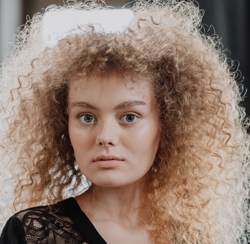
Here’s the original image that we’ll be working on:

Initialisation actions#
We first load and initialise all the necessary modules and objects that we’ll
need
1
2
3
4
5
6
7
8
| # various imports
import cv2, sys, dlib, time, math
import numpy as np
import matplotlib.pyplot as plt
from pathlib import Path
from typing import Tuple
from cv_helpers import *
from helpers import *
|
Note that cv_helpers and helpers are personal modules, mainly for debugging
/ visualisation purposes.
We then load the dlib 68 point face detector:
1
2
3
4
| path = Path(__file__).absolute().parent
predictor_path = path / "shape_predictor_68_face_landmarks.dat"
faceDetector = dlib.get_frontal_face_detector()
landmarkDetector = dlib.shape_predictor(str(predictor_path))
|
Notice that we’re taking the absolute path to the trained predictor; That’s the
correct way of opening files since this allows you to run the application
regardless your working directory. We then load the image via the cv2.imread
function, taking care of the BGR -> RGB conversion since OpenCV uses the BGR
format and finally we detect the face landmarks:
1
2
3
| im = cv2.imread(str(path / "girl-no-makeup.jpg"))
imDlib = cv2.cvtColor(im, cv2.COLOR_BGR2RGB)
landmarks = fbc.getLandmarks(faceDetector, landmarkDetector, im)
|
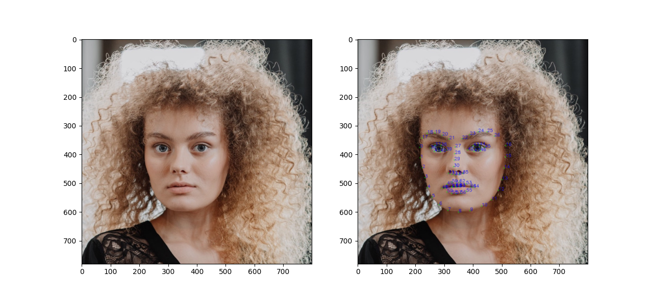
To verify that we’ve loaded the image and we’ve detected the required features
succesfully, we can plot the original image, along with it superimposed by the
detected features. To do that, we’ll make use of the following helper functions:
 1
 2
 3
 4
 5
 6
 7
 8
 9
10
11
12
13
14
15
16
17
18
19
20
21
22
23
24
25
26
27
28
29
30
31
32
33
34
35
36
37
38
39
40
41
42
43
44
45
46
47
48
49
50
51
52
53
54
55
56
57
| def mark_points_in_img(img: np.ndarray, points, inplace=True) -> np.ndarray:
"""
Each one of the points in the `points` sequence is marked by a circle and its corresponding
index in text.
"""
if not inplace:
img = img.copy()
for i, la in enumerate(points):
cv2.circle(img, la, radius=2, color=(0, 255, 0))
cv2.putText(img, str(i), la, cv2.FONT_HERSHEY_SIMPLEX, 0.5, (0, 0, 255), 1)
return img
def get_num_rows_cols(size: int, max_cols: int = 2) -> Tuple[int, int]:
"""Format `size` elements into an xy grid.
>>> get_num_rows_cols(2, max_cols=4)
(1, 2)
>>> get_num_rows_cols(4, max_cols=4)
(1, 4)
>>> get_num_rows_cols(5, max_cols=4)
(2, 4)
>>> get_num_rows_cols(10, max_cols=4)
(3, 4)
>>> get_num_rows_cols(6, max_cols=2)
(3, 2)
"""
ncols = min(size, max_cols)
if size % ncols == 0:
nrows = size // ncols
else:
nrows = int(np.ceil(size / ncols))
return nrows, ncols
def plt_imshow(*imgs, is_bgr=False):
"""
Render the given images in matplotlib. The function will automatically arrange them in a
grid layout if they are more than 2.
"""
if is_bgr:
imgs = [cv2.cvtColor(img, cv2.COLOR_BGR2RGB) for img in imgs]
if not imgs:
return
n = len(imgs)
rows, cols = get_num_rows_cols(n, max_cols=3)
fig = plt.figure(figsize=(8, 8))
for i, img in enumerate(imgs):
fig.add_subplot(rows, cols, i + 1)
plt.imshow(img)
plt.show()
|
And now to put these functions to good use:
1
2
3
| # Copy the image - keep the original intact
im1 = mark_points_in_img(imDlib, landmarks, inplace=False)
plt_imshow(imDlib, im1)
|
And here’s the result:

Applying lipstick#
To apply lipstick to the girl in the image, we follow the steps below:
- Identify the list of landmarks that comprise the lips area as well as the
area that corresponds to the mouth cavity (in case the person has slightly
opened their mouth).
- Initialise a new black image, that has the same size as the original one,
and has a solid red color at the lips.
- Slightly blur the latter, in order to soften its edges and hide potential
defects in the end result
- Finally do an alpha-blend of the two images (original girl image, lipsticks
only image) giving a higher weight to the girl
 1
 2
 3
 4
 5
 6
 7
 8
 9
10
11
12
13
14
15
16
17
18
19
20
21
22
23
24
| im_lipstick = im.copy()
# gather the indexes of the outer and inner lip cavities
lips_outer_idx = range(48, 60)
lips_outer_landmarks = [landmarks[i] for i in lips_outer_idx]
lips_inner_idx = range(60, 67)
lips_inner_landmarks = [landmarks[i] for i in lips_inner_idx]
# create lipstick-only area
im_lipstick_only = np.zeros(im_lipstick.shape, dtype=im_lipstick.dtype)
cv2.fillPoly(
im_lipstick_only, np.array([lips_outer_landmarks], np.int32), color=(0, 0, 255),
)
cv2.fillConvexPoly( # mouth cavity
im_lipstick_only, np.array(lips_inner_landmarks, np.int32), color=(0, 0, 0),
)
# do a minor blur to sotften the edges
im_lipstick_only = cv2.blur(im_lipstick_only, (5, 5))
alpha = 0.8
im_lipstick = cv2.addWeighted(im, alpha, im_lipstick_only, 1 - alpha, 0.0)
plt_imshow(im, im_lipstick, is_bgr=True)
|
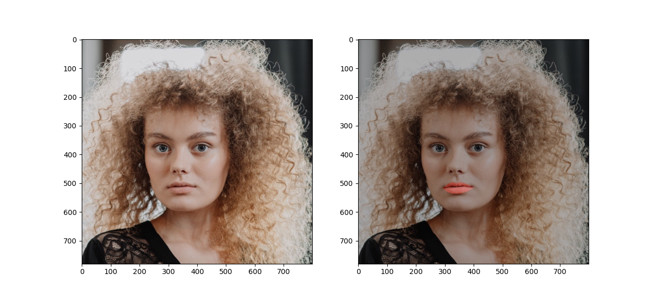
Here’s how the girl looks after having applied the lipstick:

Applying blush#
Let’s start where we left off at the previous section,
1
2
| im = im_lipstick
im = cv2.cvtColor(im, cv2.COLOR_BGR2RGB)
|
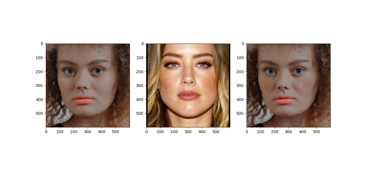
Our goal is to use a second image, let’s call it im2 which has intense blush
characteristics, and try to somehow blend it with our original image, im. To
do that, we first normalise both im and im2 to a specifc size and using
specific features and distances as reference for the normalisation. For this,
as in the first step, we will use the fbc.normalizeImagesAndLandmarks function
provided in the course material. However, instead of using the corners of the
eyes, as the points for normalisation , we will instead use the distance between
the cheek bones. Thus we add an extra class to encode this extra information,
and we change the signature of the fbc.normalizeImagesAndLandmarks function as
follows:
 1
 2
 3
 4
 5
 6
 7
 8
 9
10
11
12
13
14
15
16
17
18
19
20
21
22
| class PointsForNormalisation:
loc0: Tuple[int, int] = (0, 0)
loc1: Tuple[int, int] = (0, 0)
new_loc0: Tuple[int, int] = (0, 0)
new_loc1: Tuple[int, int] = (0, 0)
def normalizeImagesAndLandmarks(outSize: Tuple[int, int], imIn, pointsIn: np.ndarray,
points_for_normalisation:
Optional[PointsForNormalisation]=None):
...
if points_for_normalisation:
ps = points_for_normalisation
loc0 = ps.loc0
loc1 = ps.loc1
new_loc0 = ps.new_loc0
new_loc1 = ps.new_loc1
else:
# business as usual
# use corners of eyes
|
We then execute the normalisation as follows:
 1
 2
 3
 4
 5
 6
 7
 8
 9
10
11
12
13
14
15
16
17
18
19
20
21
22
23
24
25
26
27
28
29
30
31
| dst_shape = (600, 600)
landmarks_arr = np.array(landmarks)
def get_ps_for_cheeks(landmarks: np.ndarray, w, h) -> fbc.PointsForNormalisation:
ps = fbc.PointsForNormalisation()
ps.loc0 = landmarks[2]
ps.loc1 = landmarks[14]
ps.new_loc0 = (np.int(0.15 * w), np.int(h / 2))
ps.new_loc1 = (np.int(0.85 * w), np.int(h / 2))
return ps
im, landmarks_arr = fbc.normalizeImagesAndLandmarks(dst_shape, im, landmarks_arr,
get_ps_for_cheeks(landmarks_arr,
dst_shape[0],
dst_shape[1]))
landmarks = [(la[0], la[1]) for la in landmarks_arr]
assert im.shape[:-1] == dst_shape
# load, find landmarks in and reshape second image
im2_orig = cv2.imread(str(path / "makeup2.jpeg"))
im2 = cv2.cvtColor(im2, cv2.COLOR_BGR2RGB)
landmarks2 = fbc.getLandmarks(faceDetector, landmarkDetector, im2)
landmarks_arr2 = np.array(landmarks2)
im2, landmarks_arr2 = fbc.normalizeImagesAndLandmarks(dst_shape, im2, landmarks_arr2,
get_ps_for_cheeks(landmarks_arr2,
dst_shape[0],
dst_shape[1]))
landmarks2 = [(la[0], la[1]) for la in landmarks_arr2]
assert im2.shape[:-1] == dst_shape
|
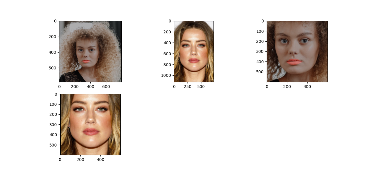
Let’s verify that the normalisation works as expected:
1
2
3
4
5
6
| plt_imshow(
cv2.cvtColor(im_lipstick, cv2.COLOR_BGR2RGB),
cv2.cvtColor(im2_orig, cv2.COLOR_BGR2RGB),
im,
im2,
)
|

Initially I thought that doing delaunay triangulation and then warping the
triangles around the cheeks area would solve it, however, as demonstrated in the
course materials, because of the different texture and skin color, this doesn’t
work and the end result doesn’t look good. I then decided to opt for two
seamless cloning operations, one for each cheek, and circular patches in the
cheeks as the mask.
Here’s how I finally implemented it:
 1
 2
 3
 4
 5
 6
 7
 8
 9
10
11
12
13
14
15
16
17
18
19
20
21
22
23
24
25
26
27
28
| # Find the center of each cheek - that's where the kernel of the blush will be
def get_cheek_loc(a: tuple, b: tuple):
# return (a[0] + b[0])//2, (a[1] + b[1])//2
xdist = b[0] - a[0]
ydist = b[1] - a[1]
x = int(a[0] + 1 / 3 * xdist)
y = int(a[1] + 1 / 3 * ydist)
return x, y
cheek1_xy = get_cheek_loc(landmarks[2], landmarks[29])
cheek2_xy = get_cheek_loc(landmarks[14], landmarks[29])
# create the masks
mask1 = np.zeros(im.shape, im.dtype)
mask2 = mask1.copy()
cv2.circle(mask1, cheek1_xy, radius=50, color=(255, 255, 255), thickness=cv2.FILLED)
cv2.circle(mask2, cheek2_xy, radius=50, color=(255, 255, 255), thickness=cv2.FILLED)
# create a copy for visualisation purposes - show where we copied pixels from
im2_ = im2.copy()
cv2.circle(im2_, cheek1_xy, radius=50, color=(255, 255, 255))
cv2.circle(im2_, cheek2_xy, radius=50, color=(255, 255, 255))
dst = cv2.seamlessClone(np.uint8(im2), im, mask1, cheek1_xy, cv2.NORMAL_CLONE)
dst = cv2.seamlessClone(np.uint8(im2), dst, mask2, cheek2_xy, cv2.NORMAL_CLONE)
plt_imshow(im, im2_, dst)
|
Here’s how the final image looks like:

As you can see, the seamless cloning operations brought a few inaccuracies from
im2 however the blush itself is visible and almost natural.
Notes#
You may need to do a few iterations selecting the image to
clone from to find one that looks as you expect. Alternatively if you found one
that you want to use but the blush is not that intense, consider editing it in a
software like gimp to increase it (e.g., by adding a new layer, painting in
it, and setting its opacity to ~60%)
Even though I demonstrated a roughly straight line between the start of this
task and the end result, that really wasn’t the case during experimentation.
Operations that you think make sense for a certain task may not, and you may
need to backtrack, think the problem differently, read the course material a few
more times, or even delete the code that you were writing for the
whole day. Might not obvious at that point in time, but this is all part of the
learning process. As you gain experience in this subject you’ll start getting a
sense of what operations should be done for each particular class of problems
and hopefully the whole process will start getting smoother.
